Dimensional analysis and similitude

Overview

Dimensional analysis and similitude provide a systematic framework for scaling fluid-mechanical behaviour from models to full-size systems. In resource-constrained African contexts where full-scale testing is often impractical or unsafe, these methods enable technicians and designers to carry out low-cost model tests, correctly interpret results, and reliably adapt solutions for diesel and gasoline systems, cooling circuits, pumps, intake/exhaust flow and other automotive fluid problems.

This topic explains the principles of scaling, the principal non-dimensional numbers used in automotive fluid mechanics, the Buckingham π method for deriving dimensionless groups, and practical guidance for designing and performing model tests with locally available materials.

Learning objectives

After studying this topic, learners will be able to:

• Explain dimensional homogeneity and the role of dimensional analysis.
• Apply the Buckingham π theorem to derive non-dimensional groups.
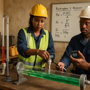
• Identify which non-dimensional numbers govern common automotive fluid problems (for example Reynolds, Froude, Mach, Weber, Prandtl).
• Decide which similarity (geometric, kinematic, dynamic) must be satisfied in a model test and why all similarity conditions cannot always be matched simultaneously.
• Design and execute low-cost model tests (pipe flow, pump, radiator or intake flow) using appropriate scaling, measurements and data reduction.
• Interpret model results and scale them to predict full-scale behaviour, highlighting uncertainties and limitations.

1. Fundamental concepts

Dimensional homogeneity

Every physically meaningful equation must be dimensionally homogeneous: every term must have the same combination of base units (mass M, length L, time T, temperature θ, electric current I, etc.). Dimensional analysis exploits this requirement to reduce the number of variables needed to describe a problem.

Example: Pressure drop Δp has units M L^-1 T^-2, velocity V has units L T^-1, density ρ is M L^-3, viscosity μ is M L^-1 T^-1.

Similitude

Similitude ensures that a model and a prototype (full-scale system) are comparable. There are three kinds:

• Geometric similarity: all linear dimensions of model and prototype are proportionally scaled by a constant λ (scale factor).
• Kinematic similarity: velocity fields are similar in non-dimensional form (trajectories of particles scale appropriately).
• Dynamic similarity: forces (inertial, viscous, gravitational, pressure) scale so dimensionless groups that govern the physics are equal in model and prototype.

Practical model testing chooses which physical effects must be replicated (dominant forces) and enforces equality of the corresponding dimensionless numbers.

2. Key non-dimensional numbers (automotive-relevant)

• Reynolds number, Re = ρ V L / μ (or V L / ν)
  • Ratio of inertial to viscous forces.
  • Governs laminar/turbulent transition and frictional losses in pipes and channels.
• Froude number, Fr = V / sqrt(g L)
  • Ratio of inertial to gravitational forces; crucial for free-surface flows (e.g., coolant surge, radiator overflow, open-channel flows).
• Mach number, Ma = V / c
  • Ratio of flow speed to speed of sound; relevant for high-speed intake/exhaust flows or nozzle flows in turbochargers.
• Weber number, We = ρ V^2 L / σ
  • Ratio of inertial to surface tension forces; important for fuel atomization and sprays.
• Strouhal number, St = f L / V
  • Characterizes unsteady oscillatory flows (vibration, pulsation).
• Euler number, Eu = Δp / (ρ V^2)
  • Pressure forces relative to inertial forces.
• Prandtl number, Pr = ν / α
  • Ratio of momentum diffusivity to thermal diffusivity; important when heat transfer and viscous effects interact (heat exchangers, radiators).
• Nusselt number, Nu = h L / k
  • Dimensionless heat transfer coefficient; used to scale convective heat transfer.

Select the numbers most relevant to the problem. For pipe flow, Re and relative roughness e/D govern friction factor; for pumps and cavitation consider cavitation number (σ) or NPSH; for radiator free-surface flow use Fr and Nu for heat transfer.

3. Buckingham π theorem — systematic derivation

Buckingham π reduces a problem of n variables with k fundamental dimensions to (n − k) independent dimensionless groups (π-groups).

Procedure:

1. List all relevant variables (including dependent and independent).
2. Express each variable’s dimensions in base units (M, L, T, θ, …).
3. Determine k, the number of fundamental dimensions present.
4. Choose k repeating variables that are dimensionally independent and do not form a π by themselves—commonly choose ρ, V, L or similar.
5. Form π-groups by combining variables so each π is dimensionless. Solve exponents to cancel dimensions.
6. Interpret the physical meaning of each π and reduce using known dimensionless numbers (Re, Fr, etc.).

Worked example: pressure drop Δp in steady incompressible flow in a circular pipe.

• Variables: Δp, ρ, μ, V, D (pipe diameter), e (roughness)
• Dimensions: Δp (M L^-1 T^-2), ρ (M L^-3), μ (M L^-1 T^-1), V (L T^-1), D (L), e (L)
• Fundamental dimensions: M, L, T → k = 3
• Choose repeating variables: ρ, V, D
• Form π-groups (sketch):
  • π1 = Δp / (ρ V^2) → pressure coefficient (Euler number)
  • π2 = μ / (ρ V D) = 1 / Re
  • π3 = e / D (relative roughness)
• Thus Δp/(ρ V^2) = f(Re, e/D). In practice this leads to friction factor correlations: f = function(Re, e/D).

4. Matching similarity — trade-offs & selection of dominant physics

Often more than one non-dimensional number matters, but it is impossible to match all simultaneously if geometric scale and available fluids/velocities are constrained. Choose which physical effects dominate:

• If viscous forces dominate (pipe flow, small-scale flow), match Reynolds number.
• If gravity/free surface is important (coolant overflow, radiator pools, water jackets with free surfaces), match Froude number.
• If surface tension controls (small droplets in injector testing), match Weber number.
• If thermal effects dominate (heat exchanger tests), consider Prandtl and Nusselt numbers.

Common trade-off: For a 1:N geometric scale, Re scales as Re_model = Re_prototype / √? No: with geometric scale λ = L_prototype / L_model:

• To match Re exactly with the same fluid, velocity must scale as V_model = V_prototype * (L_prototype / L_model) = V_prototype * λ.
• To match Fr, velocity must scale as V_model = V_prototype * sqrt(L_model / L_prototype) = V_prototype / sqrt(λ).
  Thus Fr and Re generally cannot both be matched unless other properties (viscosity, gravity) are changed. The technician must identify which effect governs the phenomenon being tested.

Illustrative numeric comparison

• Prototype: D = 100 mm, V = 2.0 m/s, ν = 1.0×10^-6 m^2/s → Re_prot = ρ V D / μ ≈ 200,000.
• Model: geometric scale λ = 4 (so D_model = 25 mm).
  • To match Re: V_model = Re_prot * ν / D_model = 200,000 * 1e-6 / 0.025 = 8.0 m/s (may be impractical).
  • To match Fr: V_model = V_prot / sqrt(λ) = 2.0 / 2 = 1.0 m/s.
    Conclusion: matching Re requires high speed; matching Fr requires lower speed. Choose based on which force balance is critical.

5. Application examples (automotive focus)

Example A — Pipe pressure drop and pump selection

• Problem: Bench-test a small-diameter sample of a diesel fuel supply line for pressure loss to predict pump power.
• Governing physics: viscous + inertial, so Re and friction factor are critical. Relative roughness e/D also matters.
• Approach: Use π groups Δp/(ρ V^2) = f(Re, e/D). If using the same fluid at model scale, adjust velocity to match Re. If speed is limited, document Re range and use charts/correlations to extrapolate to prototype Re. For turbulent flows, ensure e/D is the same in model and prototype (use same material/surface finish).

Example B — Pump cavitation (NPSH)

• Problem: Determine risk of cavitation in a fuel or cooling pump.
• Governing physics: cavitation number (σ) or NPSH relation, compressibility/phase change may be important.
• Approach: Cavitation depends on local pressure relative to vapor pressure. Maintain the same non-dimensional cavitation parameter; if matching absolute pressures is impractical, use scaled tests in a closed loop and adjust temperature/pressure in the loop to change vapor pressure (within safety limits). Visualize with low-cost transparent sections and dye or small lamp to see vapor pockets.

Example C — Radiator/heat exchanger model (free-surface and heat transfer)

• Problem: Model coolant free-surface behaviour in a radiator overflow tank; assess flow distribution between rows.
• Governing physics: free-surface flows (Fr) and heat transfer (Nu, Pr).
• Approach: Use geometric similarity and match Fr for fluid motion patterns. For heat transfer scaling, matching both Fr and Pr may be needed; if using water in both model and prototype, Pr is the same, but when different fluids are required, interpret carefully. Use simple thermocouples, inexpensive radiator cores, and dye visualization to examine flow paths.

Example D — Intake manifold flow and flow bench

• Problem: Test distribution and pressure loss in intake manifold designs using a flow bench.
• Governing physics: primarily inertial (Re high), pressure coefficients and flow separation; match Re if possible.
• Approach: Build a low-cost flow bench with a fan and pressure sensor (manometer). Use matching Re by adjusting speed or using larger scale models where possible. Use smoke or dyed air to visualize flow separation.

6. Low-cost experimental techniques and local materials

Design tests using locally available materials and simple measurement methods:

• Flow supply: garden pumps, car radiator fans, bicycle pumps, and jerrycan reservoirs.
• Test sections: clear PVC pipe, acrylic sheet, salvaged radiator cores, engine intake manifolds.
• Measuring flow:
  • Volumetric method: measure collected volume in a container over a timed interval with a stopwatch (accuracy depends on volume and time measurement).
  • Simple weirs or calibrated orifice plates cut from metal sheet.
• Measuring pressure:
  • U-tube manometer (water or water+glycerin) using transparent tubing and a scale marking.
  • Salvaged engine gauges or low-cost digital pressure sensors.
• Measuring velocity:
  • Pitot-static measurement using simple pitot tubes connected to manometer.
  • Hot-wire anemometer kits (if available) or simple vane anemometers.
• Visualisation:
  • Dye injection (water-soluble food dye for liquids).
  • Smoke sources (smoke pen, incense) for air flow visualization.
  • High-contrast background and LED lamp for photographing flow patterns.
• Heat transfer:
  • Thermocouples or digital thermometers; simple electric immersion heaters to provide constant heat flux.
• Cavitation visualization:
  • Transparent test sections with high-speed observation under safe containment.

Safety note: observe safe handling for fuels, solvents, heated fluids and pressurised apparatus. Work in well-ventilated areas, avoid open flames near fuels, and use personal protective equipment.

7. Data reduction and scaling model results to prototype

• Express measurements as dimensionless groups (π-groups). Plot dependent π (e.g., pressure coefficient or friction factor) versus relevant independent π (Re, e/D).
• Use similarity laws to scale results:
  • If Re is matched: measured dimensionless pressure coefficient directly applies to prototype.
  • If Re is not matched, use empirical correlations or theory to extrapolate; indicate uncertainties.
• Example: friction factor f measured at Re_model and e/D; use Moody chart or empirical correlations to estimate f at prototype Re and same e/D.

Uncertainty and error sources:

• Scale inaccuracies in geometry (tolerances).
• Measurement errors (timing, volume measurement, manometer resolution).
• Inability to match key dimensionless numbers (document which are matched and which are not).
• Differences in material surface roughness, fluid properties (temperature dependence).
• End effects and similarity losses near supports or instrumentation.

8. Practical assignment (competency-based)

Task: Design and perform a low-cost model test to estimate pressure drop per metre in a straight section of supply pipe for a small diesel fuel system (prototype: D = 50 mm, V ≈ 1.0 m/s). Use PVC pipe and water for safety.

Steps:

1. Identify the governing variables and derive π-groups (apply Buckingham π).
2. Choose a geometric scale λ (e.g., 2:1 or 4:1 depending on available pipe sizes).
3. Determine whether you will match Reynolds number, and calculate required model velocity; if impossible, record actual velocity and the resulting Re.
4. Build the test rig: straight pipe run (minimum 10 diameters length), inlet flow conditioning (basket strainer), flow meter (bucket + stopwatch), and manometer for pressure drop across a known length.
5. Measure volumetric flow Q (litres/sec) and compute average velocity V_model = Q / A_model; measure Δp across known length ΔL.
6. Compute Re, friction factor f (using Δp = f (L/D) (ρ V^2 / 2)), and e/D (estimate roughness).
7. Present results as f vs Re and extrapolate to prototype Re if needed using Moody-chart correlations. Discuss which similarity was preserved and the implications.

Assessment criteria:

• Correct identification of variables and derivation of π-groups (theory).
• Clear rig design and safe construction (practice).
• Accurate measurements and correct calculation of Re and f (data reduction).
• Discussion of scaling, limitations and confidence in prototype extrapolation (interpretation).

9. Common pitfalls and troubleshooting

• Trying to match too many dimensionless numbers at once — identify the dominant physics and match those numbers.
• Neglecting relative roughness e/D; scaling can change the relative importance of roughness.
• Using different fluids without accounting for changes in dimensionless numbers (viscosity, surface tension, density).
• Neglecting instrument effects and end losses — use sufficiently long test lengths and proper inlet conditioning.
• Extrapolating model results beyond the validated parameter range without appropriate caution.

10. Summary and recommended practice

• Use dimensional analysis and similitude to inform what must be matched in a model test; focus on the non-dimensional numbers that capture the dominant physics.
• Apply the Buckingham π theorem to reduce variables and identify governing parameters (Re, Fr, We, Pr, etc.).
• In resource-constrained contexts, use low-cost rigs and local materials but pay attention to matching key similarities (or documenting which are not matched) and to measurement accuracy.
• Present data in dimensionless form to allow robust scaling to full-size systems, and be explicit about uncertainties when exact similarity cannot be achieved.

End of topic.

(Recommended reading within course: worked examples in pipe flow, pump cavitation and radiator scaling; practical lab exercises using simple flow benches and manometers.)